On this page
Theory ↔ Experiment
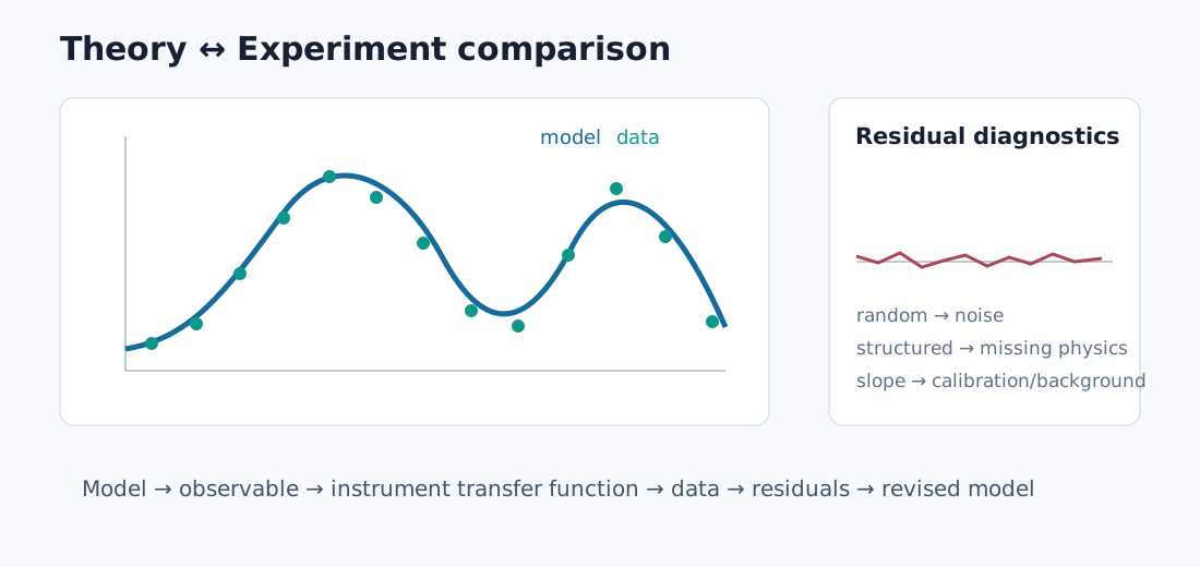
A strong technical reference should not stop at an equation or a plot. The useful chain is
\[\boxed{ \text{physical hypothesis} \rightarrow \text{model} \rightarrow \text{observable} \rightarrow \text{instrument transfer function} \rightarrow \text{data} \rightarrow \text{residuals} }\]1. Start with the observable
Ask first: what does the instrument actually output?
Examples:
- VNA → complex wave ratio;
- photodetector → photocurrent/voltage, not atomic population directly;
- spectrum analyzer → filtered/detected spectral power;
- oscilloscope → bandwidth-limited voltage waveform;
- atomic receiver → optical transmission/phase/polarization encoding an RF-driven susceptibility.
2. Separate physics from readout
For a Rydberg current experiment, for example:
\[\text{atomic excitation} \rightarrow \text{ionization} \rightarrow \text{particle transport} \rightarrow \text{Shockley–Ramo current} \rightarrow Z_T(\omega) \rightarrow V_{scope}.\]If the final voltage disagrees with theory, the disagreement can live in any layer.
3. Add realism in controlled steps
Do not begin with every complication. Use a ladder:
- ideal analytic model;
- measured geometry;
- measured drive amplitudes;
- finite linewidth/loss;
- spatial averaging;
- instrumental bandwidth;
- temperature/drift;
- interactions/nonlinearity;
- uncertainty propagation.
At each step, ask whether the change improves the particular residual seen in data.
4. Compare shapes before amplitudes
A useful debugging order is:
- peak position;
- symmetry/asymmetry;
- linewidth;
- number of peaks;
- relative amplitudes;
- absolute scale.
Absolute amplitude is often the last thing to trust because it accumulates calibration errors from many layers.
5. Plot residuals
For data $y_i$ and model $m_i$,
\[r_i=y_i-m_i.\]Residual structure is diagnostic:
- random scatter → noise-dominated;
- slope → calibration/background error;
- alternating structure → frequency-axis or phase issue;
- broadened central residual → missing linewidth/spatial averaging;
- systematic side features → missing states/modes/coupling pathways.
6. Use dimensionless comparisons
Before fitting many parameters, compare regime ratios such as
\[\Omega/\Gamma,\qquad \Omega/\Delta,\qquad ka,\qquad \omega_c/\nu_{coll},\qquad R/R_{FF}.\]These ratios often tell you what physics can plausibly matter.
7. Calibrate independently where possible
A parameter measured independently should not also be freely fitted unless you are explicitly testing its calibration.
Examples:
- RF field from AT calibration;
- laser power/waist → optical Rabi estimate;
- photodetector transfer function measured separately;
- magnetic field from atomic resonance;
- cable loss from VNA/power calibration.
8. Falsification tests
A good model should predict what happens when you deliberately change a control parameter that was not used to fit it.
Examples:
- reverse $B$;
- rotate polarization;
- change vapor-cell position;
- change beam waist;
- vary detector bandwidth;
- switch a Floquet replica order/basis size;
- change antenna distance from near to far field.
9. Theory ↔ experiment templates
Antenna
Maxwell/full-wave model → current distribution → far-field pattern → chamber transfer/calibration → measured pattern.
RF receiver
signal source → channel → antenna/front end → gain/noise/nonlinearity → demodulator → EVM/BER.
Atomic sensor
Hamiltonian → density matrix/Floquet → susceptibility → propagation → photodetection → electronics → measured spectrum/beat note.
Charged-particle detector
field map → particle transport → weighting field → induced current → amplifier response → waveform.
10. A reusable comparison figure
For publication-quality theory/experiment comparisons, show whenever possible:
- same axes and units;
- shared color scale;
- measured and simulated linewidths;
- residual panel or difference map;
- independently measured parameters listed in caption/table;
- fitted parameters explicitly labeled;
- uncertainty or repeatability indication.
See Measurements & Instruments, Simulation Library, and Scaling Laws.