On this page
Atomic Ground-State Magnetic-Field Sensing
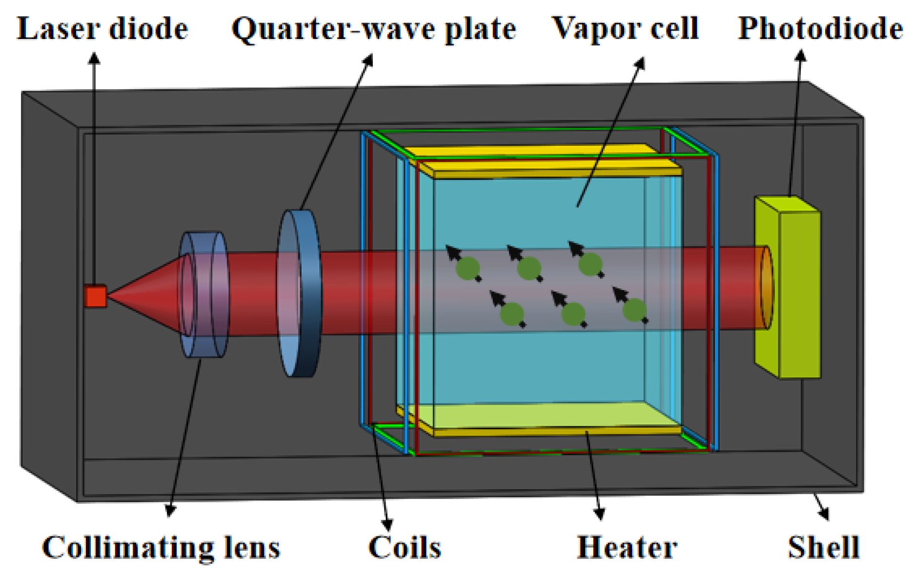
Atomic ground-state magnetometers use the Zeeman response and coherent spin dynamics of long-lived ground-state atomic levels to measure magnetic fields. Alkali-metal atoms such as cesium (Cs), rubidium (Rb), and potassium (K) are especially useful because optical pumping and optical readout provide efficient access to their ground-state electron/nuclear spin polarization.
Unlike Rydberg electrometry, where highly excited states provide enormous electric-dipole response, ground-state atomic magnetometry primarily exploits the magnetic interaction
\[\boxed{H_B=-\boldsymbol\mu\cdot\mathbf B}.\]The basic transduction chain is
\[\boxed{ \mathbf B \rightarrow \text{Zeeman splitting / spin precession} \rightarrow \text{atomic coherence} \rightarrow \text{optical signal} \rightarrow V_{PD} }.\]1. Alkali ground states
For an alkali atom, the electronic ground state is typically
\[nS_{1/2}.\]The electron angular momentum $\mathbf J$ couples to nuclear spin $\mathbf I$ to form
\[\mathbf F=\mathbf I+\mathbf J.\]For cesium-133,
\[I=\frac72,\]and the $6S_{1/2}$ ground state has hyperfine manifolds
\[F=3,4.\]The zero-field hyperfine splitting is approximately
\[9.192631770\ \text{GHz},\]which defines the SI second through the cesium-133 ground-state hyperfine transition.
Each $F$ manifold contains magnetic sublevels
\[m_F=-F,-F+1,\ldots,+F.\]These magnetic sublevels are the basis of many atomic magnetometers.
2. Zeeman effect
In a sufficiently weak magnetic field, the first-order ground-state Zeeman shift is
\[\boxed{ \Delta E_{F,m_F}=g_F\mu_Bm_FB }\]and adjacent Zeeman levels are separated by
\[\Delta E=g_F\mu_BB.\]The corresponding angular frequency is
\[\boxed{ \omega_L=\gamma B }\]where $\gamma$ is the effective gyromagnetic ratio.
Thus measuring a frequency can directly determine magnetic field:
\[\boxed{ B=\frac{\omega_L}{\gamma}. }\]This frequency-to-field conversion is one reason atomic magnetometers can provide highly stable and fundamentally referenced measurements.
3. Larmor precession

An atomic magnetic moment in a magnetic field experiences torque,
\[\boldsymbol\tau=\boldsymbol\mu\times\mathbf B.\]The collective atomic spin therefore precesses around the magnetic field.
Semiclassically,
\[\frac{d\mathbf F}{dt} = \gamma\mathbf F\times\mathbf B.\]The precession frequency is the Larmor frequency
\[f_L=\frac{\gamma}{2\pi}B.\]Ground-state magnetometry is therefore closely related to NMR, ESR, gyroscopes, and classical magnetic resonance.
4. Breit–Rabi equation
The simple linear Zeeman expression eventually fails as the magnetic interaction becomes comparable to the hyperfine interaction.
For alkali $S_{1/2}$ ground states, the Breit–Rabi equation describes the hyperfine-Zeeman energies over a much wider magnetic-field range.
A standard form is
\[E_{F=I\pm1/2,m_F} = -\frac{\Delta E_{hfs}}{2(2I+1)} + g_I\mu_Bm_FB \pm \frac{\Delta E_{hfs}}{2} \sqrt{ 1+ \frac{4m_F}{2I+1}x+x^2 },\]with
\[x= \frac{(g_J-g_I)\mu_BB} {\Delta E_{hfs}}.\]The Breit–Rabi relation is essential when modeling nonlinear Zeeman effects or extending the dynamic range beyond the weak-field approximation.
5. Optical pumping
Circularly polarized resonant light transfers angular momentum from photons to atoms.
Repeated absorption and spontaneous emission can accumulate population in selected magnetic sublevels and create a macroscopic spin polarization
\[\mathbf P = \frac{\langle\mathbf F\rangle}{F}.\]This converts an initially almost unpolarized thermal vapor into an ensemble with a measurable collective magnetic moment.
The basic process is
\[\boxed{ \text{polarized light} \rightarrow \text{atomic spin polarization} \rightarrow \text{magnetic-field evolution} \rightarrow \text{optical readout}. }\]6. Optical orientation and alignment
Optical pumping can create different polarization moments.
Orientation corresponds roughly to a preferred spin direction and is a rank-1 polarization moment.
Alignment corresponds to anisotropic population without necessarily having a net spin direction and is associated with rank-2 polarization.
Different magnetometer configurations can detect orientation, alignment, or higher-order polarization moments.
7. Bloch equations
A useful semiclassical model for collective magnetization is
\[\frac{d\mathbf M}{dt} = \gamma\mathbf M\times\mathbf B - \frac{M_x\hat x+M_y\hat y}{T_2} - \frac{(M_z-M_0)\hat z}{T_1}.\]Here
- $T_1$ describes longitudinal relaxation,
- $T_2$ describes transverse coherence decay.
The magnetic-resonance linewidth scales approximately as
\[\Delta f\sim\frac{1}{\pi T_2}.\]Long ground-state coherence times are therefore central to high magnetic sensitivity.
8. Optically pumped magnetometer (OPM)
A basic OPM contains
alkali vapor cell → pump laser → magnetic-field interaction → probe/readout → photodetector → demodulation.
A bias field can establish a Larmor frequency while a transverse RF magnetic field drives transitions between Zeeman sublevels.
At resonance,
\[\omega_{RF}\approx\omega_L.\]The optical transmission or polarization then becomes modulated at the magnetic resonance.
See the broader Optically Pumped Atomic Magnetometer page.
9. Mx magnetometer
In an Mx magnetometer, the static field is oriented at an angle to the optical axis and an RF magnetic field drives coherent spin precession.
The resonance frequency gives
\[B=\frac{2\pi f_L}{\gamma}.\]The phase response around resonance can provide an especially useful error signal for closed-loop operation.
10. Mz magnetometer
In an Mz configuration, the optical pumping and static magnetic field are commonly arranged along the same axis.
A transverse RF field drives magnetic resonance, which changes longitudinal spin polarization and therefore optical absorption.
Mz sensors are conceptually simple and have been widely used in scalar magnetometry.
11. Bell–Bloom magnetometer
Instead of applying a separate RF magnetic field, the optical pumping itself can be modulated.
If the pump modulation frequency approaches the Larmor frequency,
\[\omega_{mod}\approx\omega_L,\]the modulated light synchronously drives the atomic spin.
This is known as Bell–Bloom optical pumping.
It replaces an RF excitation coil with an optically modulated drive and is widely used in modern atomic magnetometry.
12. Nonlinear magneto-optical rotation (NMOR)
Near-resonant polarized light can create ground-state coherence while the magnetic field rotates the atomic polarization.
The resulting medium rotates the polarization plane of transmitted light.
The optical rotation angle can be extremely sensitive to magnetic field.
NMOR combines optical pumping, ground-state coherence, Zeeman evolution, and polarization-sensitive optical detection.
13. Faraday rotation readout
For linearly polarized probe light, the two circular components $\sigma^+$ and $\sigma^-$ can experience different refractive indices.
The polarization rotation is approximately
\[\theta = \frac{kL}{2}(n_+-n_-).\]Because $n_+-n_-$ depends on atomic spin polarization, measuring optical rotation provides a sensitive, often nearly non-destructive readout of spin precession.
Balanced polarimetry is frequently used.
14. SERF magnetometer
The spin-exchange relaxation-free (SERF) regime enables some of the highest sensitivities achieved by atomic magnetometers.
Spin-exchange collisions normally cause relaxation. At sufficiently high alkali density and sufficiently low magnetic field, however, the spin-exchange rate becomes much faster than the Larmor precession frequency:
\[\boxed{ R_{SE}\gg\omega_L. }\]The rapid collisions average out much of the spin-exchange broadening.
SERF operation typically requires:
- high alkali vapor density;
- elevated cell temperature;
- very small residual magnetic field;
- magnetic shielding and compensation coils.
Sensitivities can reach the femtotesla-per-root-hertz regime and below in optimized laboratory systems.
15. Spin-exchange collisions
Two alkali atoms can exchange electron-spin polarization during a collision.
The process conserves total angular momentum but redistributes population and coherence among hyperfine states.
Depending on magnetic field and collision rate, spin exchange can either limit linewidth or, in the SERF regime, become effectively averaged.
16. Spin-destruction collisions
Unlike spin exchange, spin-destruction collisions irreversibly remove atomic polarization.
Sources include:
- alkali–alkali collisions;
- alkali–buffer-gas collisions;
- collisions with cell walls.
Spin-destruction rate sets an important ultimate limit on ground-state coherence time.
17. Buffer gas
Buffer gases such as N$_2$, He, or noble gases reduce rapid diffusion of alkali atoms to the cell walls.
They can therefore increase interaction time and ground-state coherence.
However, buffer gas also introduces pressure broadening and frequency shifts of optical transitions.
The optimum pressure depends on sensor geometry and operating mode.
18. Anti-relaxation wall coatings
Paraffin-like and other anti-relaxation coatings allow alkali atoms to collide with the cell wall many times while retaining spin polarization.
Coated cells can therefore achieve long coherence times without high buffer-gas pressure.
This is especially valuable for low-frequency and compact magnetometers.
19. Scalar magnetometry
A scalar magnetometer measures approximately
\[|\mathbf B|.\]Because the Larmor frequency depends primarily on field magnitude, frequency-based OPMs naturally operate as scalar sensors.
This can reduce sensitivity to sensor orientation, although heading errors and nonlinear effects remain possible.
20. Vector magnetometry
A vector magnetometer seeks
\[B_x,\quad B_y,\quad B_z.\]Vector information can be obtained using multiple optical axes, multiple modulation directions, polarization-dependent signals, controlled bias fields, or simultaneous measurement of different atomic observables.
Atomic vector magnetometry is useful for navigation, biomagnetism, magnetic mapping, and field characterization.
21. RF atomic magnetometry
Ground-state Zeeman transitions can directly detect oscillating magnetic fields.
For
\[\mathbf B(t) = B_0\hat z+ B_1\cos(\omega t)\hat x,\]the transverse field drives magnetic-dipole transitions when
\[\omega\approx\gamma B_0.\]The interaction Hamiltonian is
\[H_{RF} = -\boldsymbol\mu\cdot\mathbf B_{RF}.\]The RF Rabi frequency is
\[\Omega_{RF} = \frac{ |\langle f|\boldsymbol\mu\cdot\mathbf B_{RF}|i\rangle| }{\hbar}.\]Thus a ground-state atom can function as an RF magnetic-field receiver.
22. DC versus AC magnetic sensing
Ground-state sensors can measure both:
DC/quasi-static fields: infer $B$ from Larmor frequency, optical rotation, or spin orientation.
AC/RF fields: resonantly drive Zeeman transitions and measure amplitude, frequency, phase, or polarization.
The operating frequency can often be tuned simply by changing the bias field.
23. Magnetic resonance linewidth and sensitivity
For a resonance of width $\Gamma$ and signal-to-noise ratio SNR, a useful qualitative scaling is
\[\delta B \propto \frac{\Gamma}{\gamma\,\mathrm{SNR}}.\]Thus sensitivity improves with:
- narrow magnetic resonance;
- long coherence time;
- large atomic polarization;
- high optical signal-to-noise;
- high atom number;
- low technical noise.
24. Atomic projection noise
For $N$ uncorrelated atoms measured over coherence time $T_2$, the standard quantum limit has a characteristic scaling
\[\delta B \sim \frac{1}{\gamma\sqrt{NT_2t}},\]where $t$ is total integration time, up to factors depending on protocol.
This illustrates why large atom number and long ground-state coherence are powerful.
Spin squeezing and entanglement can in principle surpass the uncorrelated-atom limit.
25. Photon shot noise
Optical readout also has photon shot noise.
Increasing probe power can reduce photon-shot-noise-limited uncertainty, but excessive optical power produces power broadening, AC Stark shifts, and additional optical pumping.
Sensitivity therefore requires optimization rather than simply increasing laser power.
26. Magnetic shielding
Environmental magnetic noise can greatly exceed the intrinsic atomic noise.
High-sensitivity systems therefore often use multiple layers of high-permeability magnetic shielding.
Internal coils provide:
- residual-field cancellation;
- calibrated bias fields;
- field gradients;
- test signals.
SERF sensors are particularly dependent on strong field suppression.
27. Magnetic-field gradients
If the magnetic field varies across the vapor cell, different atoms precess at different frequencies.
This causes inhomogeneous dephasing and broadening.
For position-dependent field
\[B(\mathbf r)=B_0+\delta B(\mathbf r),\]the observed signal is an average over a distribution of Larmor frequencies.
Gradient compensation can therefore substantially improve coherence.
28. Gradiometry
Two or more atomic sensors can measure field differences:
\[\frac{\partial B}{\partial x} \approx \frac{B_2-B_1}{d}.\]Common-mode environmental magnetic noise can cancel while nearby magnetic sources remain visible.
Atomic gradiometers are important for biomagnetism, geophysics, magnetic anomaly detection, and unshielded sensing.
29. Heading error
The response of an atomic magnetometer can depend on the angle between the magnetic field, optical polarization, and sensor axes.
Nonlinear Zeeman shifts, unresolved resonances, optical pumping, tensor light shifts, and polarization imperfections can produce orientation-dependent systematic errors known as heading errors.
This is important for Earth-field magnetometry and navigation.
30. Light shifts
Off-resonant optical fields can shift ground-state energies through the AC Stark effect.
A pump or probe laser can therefore generate an effective magnetic-field-like systematic shift.
Vector light shifts can depend on polarization and propagation direction.
Laser detuning, intensity, and polarization must consequently be controlled in precision magnetometry.
31. Nonlinear Zeeman effect
At larger magnetic fields, adjacent $m_F$ transitions are no longer equally spaced.
The Breit–Rabi equation predicts the nonlinear spectrum.
Consequences include:
- resonance splitting;
- line-shape distortion;
- heading error;
- reduced scalar accuracy;
- multiple RF resonances.
This effect becomes particularly relevant near Earth’s field compared with near-zero-field SERF operation.
32. Coherent population trapping and CPT magnetometry
Ground-state hyperfine or Zeeman coherences can be prepared using two coherent optical fields.
A dark resonance occurs when the two-photon frequency difference matches the ground-state splitting.
Magnetic fields shift the participating levels and therefore shift the CPT resonance.
CPT thus provides another route to magnetic sensing closely related to EIT.
33. EIT-based ground-state magnetometry
A lambda-type EIT system can use two ground-state Zeeman or hyperfine levels coupled through a common excited state.
The magnetic field shifts the ground-state two-photon resonance:
\[\delta_{2\gamma}(B) \propto (g_{F_2}m_{F_2}-g_{F_1}m_{F_1})\mu_BB/\hbar.\]Measuring the displacement, splitting, or phase of the EIT resonance provides a magnetic-field estimate.
This is conceptually distinct from Rydberg EIT because the sensing interaction occurs primarily in the long-lived ground-state coherence.
34. Microwave hyperfine magnetometry
Microwave transitions between ground-state hyperfine manifolds can also sense magnetic field through their Zeeman dependence.
For Cs, transitions near the 9.192 GHz clock splitting can be interrogated while magnetic fields shift non-clock transitions.
This connects atomic magnetometry directly to atomic clocks and microwave spectroscopy.
35. Ground-state versus Rydberg magnetic sensing
| Ground-state atomic sensing | Rydberg-state sensing |
|---|---|
| Long-lived spin coherence | Highly excited electronic state |
| Magnetic-dipole response | Strong electric-dipole response |
| Zeeman/Larmor physics | Stark, Zeeman and RF-dressed physics |
| DC to RF magnetic fields | Primarily RF electric fields; magnetic sensing also possible |
| fT-level magnetic sensitivity possible | Excellent RF E-field sensitivity and SI traceability |
| OPM/SERF/CPT/NMOR | Rydberg EIT/AT/Floquet |
The two approaches are complementary.
A useful comparison is
\[\boxed{ \text{Ground state: }\mathbf B \rightarrow -\boldsymbol\mu\cdot\mathbf B \rightarrow \text{spin coherence} }\]versus
\[\boxed{ \text{Rydberg state: }\mathbf E \rightarrow -\mathbf d\cdot\mathbf E \rightarrow \text{Rydberg coherence}. }\]36. Ground-state sensing combined with Rydberg EIT
A particularly interesting hybrid strategy is to use different parts of the same atom as complementary sensors.
Ground-state Zeeman structure can provide magnetic-field information while Rydberg levels provide strong RF electric-field response.
In a sufficiently complete multilevel model,
\[H= H_{hfs} + H_Z + H_{opt} + H_{Rydberg} + H_{RF}.\]This allows simultaneous or correlated sensing of electric and magnetic fields and helps separate magnetic systematic shifts from RF electric-field effects.
37. Halbach permanent-magnet arrays
A Halbach array is a deliberately arranged sequence of permanent magnets whose magnetization direction rotates from one magnet segment to the next. The geometry reinforces the magnetic field on one side of the array while suppressing it on the opposite side.
For an ideal continuously varying planar Halbach magnetization, one can represent the rotating magnetization schematically as
$ \mathbf M(x) = M_0[ \cos(kx)\hat x+ \sin(kx)\hat y ]. $
The resulting field is strongly concentrated on one side and approximately decays away from the array as
$ B(y)\propto e^{-ky}. $
This is sometimes described as a one-sided magnetic flux structure.

Why Halbach arrays are useful for atomic sensing
Atomic magnetometers often require a stable bias field but may also benefit from compactness, low electrical power, and reduced external stray field. A Halbach structure can provide:
- a strong permanent bias field without a continuously powered coil;
- reduced field on the exterior side of the magnet assembly;
- compact magnetic circuits;
- cylindrical geometries with a strong internal field;
- mechanically stable field generation;
- reduced power dissipation near a vapor cell.
This can be useful for portable atomic sensors, compact spectroscopy systems, microwave hyperfine experiments, and experiments requiring a permanent quantization field.
Cylindrical Halbach array
A particularly important configuration is the Halbach cylinder, in which magnetization rotates around a cylindrical shell.
An ideal infinitely long $p=1$ Halbach cylinder produces an approximately uniform transverse magnetic field inside the bore while suppressing the external field.
For an ideal cylindrical permanent magnet with inner radius $R_i$, outer radius $R_o$, and remanent flux density $B_r$, a commonly quoted ideal result is
$ \boxed{ B_{bore}\approx B_r\ln\left(\frac{R_o}{R_i}\right) } $
for the dipole Halbach configuration, subject to ideal material and infinite-length assumptions.
Real arrays use discrete magnet blocks, finite length, and nonideal material properties, so the actual field and homogeneity must normally be calculated numerically and verified experimentally.
Segmented Halbach arrays
A continuous rotating magnetization is difficult to manufacture. Practical arrays therefore use $N$ discrete permanent-magnet segments.
Increasing the number of segments makes the magnetization distribution more closely approximate the ideal continuous Halbach pattern and generally improves field quality, at the cost of mechanical complexity.
Common magnet materials include NdFeB and SmCo.
Field homogeneity
For precision atomic spectroscopy, field magnitude alone is insufficient. The spatial variation across the atomic vapor is critical:
$ B(\mathbf r)=B_0+\delta B(\mathbf r). $
A gradient produces a distribution of Larmor frequencies,
$ \omega_L(\mathbf r)=\gamma B(\mathbf r), $
which broadens the atomic resonance and reduces coherence.
A useful homogeneity measure over the sensing volume is
$ \frac{\Delta B}{B_0}. $
Consequently a Halbach array intended for atomic sensing should be optimized for field uniformity over the vapor-cell volume, not merely maximum central field.
Halbach array versus Helmholtz coils
| Halbach array | Helmholtz coils |
|---|---|
| Permanent field | Electrically generated field |
| Essentially zero steady-state electrical power | Requires current |
| Compact high-field designs possible | Excellent tunability |
| Limited electronic tunability | Field easily swept/reversed |
| Temperature dependence of magnets | Current-source stability matters |
| Mechanical alignment important | Coil geometry/alignment important |
| Can suppress external stray field | External field generally not inherently suppressed |
A useful hybrid architecture is
$ \boxed{ \text{Halbach array} + \text{small trim coils} } $
where the permanent magnets provide the main bias field and low-power coils provide fine tuning, gradient compensation, modulation, or field reversal.
Temperature stability
Permanent-magnet remanence varies with temperature,
$ B_r=B_r(T). $
Therefore a precision Halbach bias field can drift with ambient temperature. Temperature coefficients depend strongly on magnet material and grade.
Possible mitigation includes:
- temperature stabilization;
- thermally compensated magnet combinations;
- SmCo where appropriate for improved thermal stability;
- field calibration using the atomic resonance itself;
- trim coils under feedback control.
Magnetic shielding and Halbach arrays
A Halbach structure can reduce stray field but does not automatically shield the atoms from environmental magnetic fields.
High-sensitivity experiments may still require high-permeability shielding around the magnet/vapor-cell assembly.
Care is also required because nearby magnetic shielding changes the boundary conditions and can perturb the Halbach field.
The complete magnetic structure should therefore be modeled together when high field accuracy is required.
Numerical modeling
Finite-element magnetostatic simulation is especially useful for realistic Halbach assemblies.
Solve
$ \nabla\cdot\mathbf B=0, \qquad \nabla\times\mathbf H=\mathbf J, $
with
$ \mathbf B=\mu_0(\mathbf H+\mathbf M) $
inside the permanent magnets.
Useful outputs include:
- $B_x,B_y,B_z$ throughout the vapor cell;
-
field magnitude $ \mathbf B $; - first- and higher-order gradients;
- field-angle variation;
- sensitivity to magnet-position errors;
- sensitivity to magnetization-angle errors;
- finite-length/end effects;
- effects of shields and nearby magnetic materials.
For an atomic sensor, the most meaningful simulation output is often the distribution of Zeeman shifts across the illuminated atomic volume rather than simply a magnetic-field map.
Connection to Rydberg EIT
A Halbach array can also provide a controlled quantization field for Rydberg-EIT experiments.
The chain becomes
$ \boxed{ \text{Halbach field} \rightarrow \text{Zeeman-resolved }m_F/m_J\text{ structure} \rightarrow \text{polarization-selective optical/RF coupling} \rightarrow \text{EIT / AT / Floquet spectrum}. } $
A sufficiently uniform bias field can define the quantization axis and separate magnetic sublevels. Conversely, excessive gradients broaden the Zeeman-resolved EIT peaks and complicate RF polarization and vector-field measurements.
For experiments combining ground-state and Rydberg sensing, a compact Halbach-plus-trim-coil assembly could therefore provide a common, stable quantization field while retaining fine electronic control.
Applications beyond atomic sensing
Halbach arrays are widely used in:
- compact permanent-magnet MRI and NMR;
- particle accelerators and undulators;
- electric motors and generators;
- magnetic bearings;
- magnetic levitation;
- magnetic separators;
- laboratory bias-field sources;
- portable spectroscopy instruments.
The central design principle is
$ \boxed{ \text{rotating magnetization} \rightarrow \text{constructive field on one side} + \text{destructive field on the other}. } $
38. Applications
Ground-state atomic magnetometers are used or studied for:
- magnetoencephalography (MEG);
- magnetocardiography (MCG);
- fetal biomagnetism;
- NMR and zero/ultralow-field NMR;
- geophysical surveys;
- geomagnetic monitoring;
- navigation;
- magnetic anomaly detection;
- current imaging;
- materials characterization;
- unexploded-ordnance detection;
- fundamental-symmetry searches;
- searches for exotic spin-dependent interactions;
- space magnetometry;
- RF magnetic-field detection;
- magnetic gradiometry.
Quick reference
\[\boxed{ H_B=-\boldsymbol\mu\cdot\mathbf B }\] \[\boxed{ \Delta E_Z=g_F\mu_Bm_FB }\] \[\boxed{ \omega_L=\gamma B }\] \[\boxed{ \frac{d\mathbf M}{dt} = \gamma\mathbf M\times\mathbf B - \text{relaxation} + \text{optical pumping} }\]The shortest physical picture is
\[\boxed{ \text{pump the spins} \rightarrow \text{let }\mathbf B\text{ rotate/shift them} \rightarrow \text{read the spins optically}. }\]References and further reading
- D. Budker and M. Romalis, “Optical Magnetometry,” Nature Physics 3, 227–234 (2007). https://doi.org/10.1038/nphys566
- D. Budker and D. F. J. Kimball, Optical Magnetometry, Cambridge University Press (2013).
- W. Happer, “Optical Pumping,” Reviews of Modern Physics 44, 169 (1972). https://doi.org/10.1103/RevModPhys.44.169
- W. Happer and H. Tang, “Spin-Exchange Shift and Narrowing of Magnetic Resonance Lines in Optically Pumped Alkali Vapors,” Physical Review Letters 31, 273 (1973). https://doi.org/10.1103/PhysRevLett.31.273
- J. C. Allred et al., “High-Sensitivity Atomic Magnetometer Unaffected by Spin-Exchange Relaxation,” Physical Review Letters 89, 130801 (2002). https://doi.org/10.1103/PhysRevLett.89.130801
- I. K. Kominis et al., “A subfemtotesla multichannel atomic magnetometer,” Nature 422, 596–599 (2003). https://doi.org/10.1038/nature01484
- J. Kitching, “Chip-scale atomic devices,” Applied Physics Reviews 5, 031302 (2018). https://doi.org/10.1063/1.5026238
- D. Budker et al., “Resonant nonlinear magneto-optical effects in atoms,” Reviews of Modern Physics 74, 1153 (2002). https://doi.org/10.1103/RevModPhys.74.1153
- E. B. Alexandrov, M. V. Balabas, A. K. Vershovskii, A. S. Pazgalev, and A. K. Yakobson, literature on optically pumped alkali-vapor magnetometers.
- H. B. Dang, A. C. Maloof, and M. V. Romalis, “Ultrahigh sensitivity magnetic field and magnetization measurements with an atomic magnetometer,” Applied Physics Letters 97, 151110 (2010). https://doi.org/10.1063/1.3491215
- T. W. Kornack et al., literature on SERF magnetometry and magnetic gradiometry.
- NIST, chip-scale atomic magnetometer and atomic-sensor research — https://www.nist.gov/
- C. L. Degen, F. Reinhard, and P. Cappellaro, “Quantum sensing,” Reviews of Modern Physics 89, 035002 (2017). https://doi.org/10.1103/RevModPhys.89.035002
- K. Halbach, “Design of permanent multipole magnets with oriented rare earth cobalt material,” Nuclear Instruments and Methods 169, 1–10 (1980). https://doi.org/10.1016/0029-554X(80)90094-4
- J. C. Mallinson, “One-sided fluxes — A magnetic curiosity?” IEEE Transactions on Magnetics 9, 678–682 (1973). https://doi.org/10.1109/TMAG.1973.1067714
- R. Bjørk et al., “The efficiency and the demagnetization field of a general Halbach cylinder,” Journal of Applied Physics 104, 013910 (2008). https://doi.org/10.1063/1.2952537
- Permanent-magnet Halbach geometries are also widely developed in compact NMR/MRI literature, where bore-field homogeneity and finite-length optimization closely parallel atomic-spectroscopy requirements.
Related pages
- Optically Pumped Atomic Magnetometer
- Semiclassical Quantum Optics for Rydberg EIT
- Hydrogen Maser
- Lorentz Force
- Fundamental Equations