On this page
Optically Pumped Atomic Magnetometer
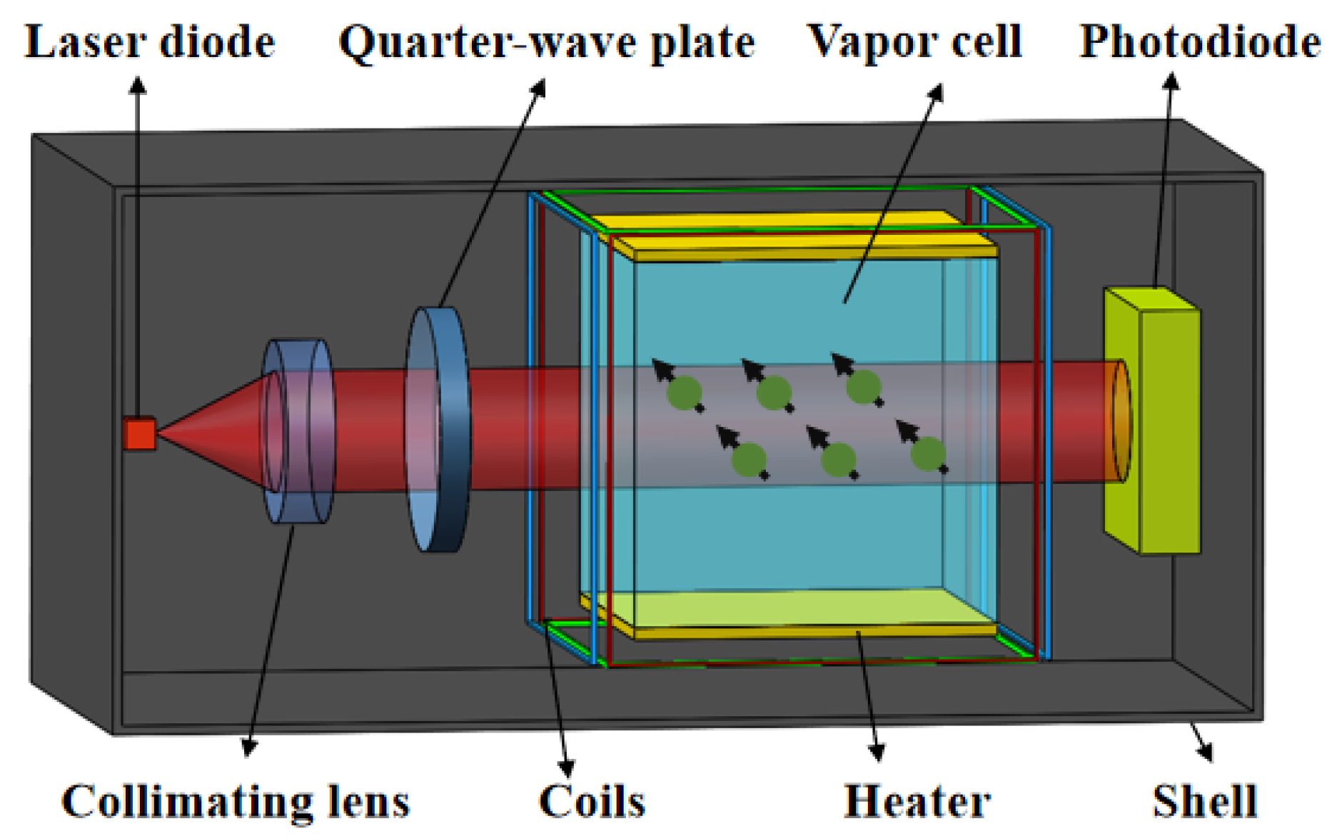
An optically pumped atomic magnetometer (OPM) is one of the clearest examples of a device in which quantum states, optics, RF engineering, magnetic fields, feedback electronics, and precision measurement operate as one system.
The essential idea is simple:
optical pumping → polarized atomic spins → magnetic-field-driven Larmor precession → optical readout → magnetic-field estimate.
It is therefore a natural companion to the hydrogen maser. A maser uses an atomic transition to generate or stabilize a microwave frequency; an atomic magnetometer uses the field-dependent evolution of atomic spins to infer an external magnetic field.
1. Quantum basis: atomic magnetic moment
Atoms with angular momentum carry a magnetic moment. In a magnetic field, the interaction is
\[H_B=-\boldsymbol{\mu}\cdot\mathbf B.\]For a hyperfine level with total angular momentum $F$, the first-order Zeeman shift is approximately
\[\Delta E_{F,m_F}=g_F\mu_B m_F B,\]where $g_F$ is the hyperfine Landé factor and $\mu_B$ is the Bohr magneton.
Adjacent Zeeman sublevels are therefore separated by a magnetic-field-dependent frequency. The collective atomic polarization precesses around the magnetic field at the Larmor frequency
\[\boxed{\omega_L=\gamma B}\]or
\[\boxed{f_L=\frac{\gamma}{2\pi}B},\]where $\gamma$ is the relevant gyromagnetic ratio.
This equation is the fundamental transduction relation of an atomic magnetometer:
\[\boxed{\text{frequency} \longleftrightarrow \text{magnetic field}.}\]NIST describes atomic magnetometers as relying on fundamental atomic properties to translate magnetic field into a measurable Larmor frequency.
2. Typical atomic species
Common vapor-cell magnetometers use alkali atoms such as
- cesium (Cs),
- rubidium (Rb),
- potassium (K).
These atoms are attractive because their single valence electron gives accessible optical transitions and a well-understood ground-state spin structure.
A practical vapor-cell instrument may contain the alkali vapor together with buffer gas or a wall coating to reduce spin relaxation.
3. Optical pumping — preparing the quantum state
Circularly polarized resonant or near-resonant light transfers angular momentum from photons to the atoms. Repeated absorption and spontaneous-emission cycles redistribute the ground-state populations and create a spin-polarized ensemble.
Schematically,
\[\text{polarized photons} \rightarrow \text{atomic angular momentum} \rightarrow \text{macroscopic spin polarization}.\]Instead of measuring one atom, an OPM usually measures the coherent response of a large ensemble.
The polarization can be represented by a collective spin or magnetization vector $\mathbf P$ or $\mathbf M$.
4. Larmor precession
Once polarized, the atomic spins experience a torque in an external magnetic field:
\[\frac{d\mathbf S}{dt}=\boldsymbol{\mu}\times\mathbf B.\]The ensemble consequently precesses about the magnetic-field direction.
This is the atomic analogue of gyroscopic precession, but here the object undergoing precession is a quantum angular-momentum ensemble.
If an RF magnetic field is applied transverse to the bias field,
\[\mathbf B(t)=B_0\hat z+B_1\cos(\omega t)\hat x,\]a resonant response occurs when
\[\boxed{\omega\approx\omega_L=\gamma B_0.}\]This is where atomic magnetometry connects directly to RF engineering.
5. RF-driven atomic magnetometer
In the classic $M_x$ configuration, atoms are optically polarized and an oscillating transverse magnetic field drives the spin system near the Larmor resonance.
The RF field couples magnetic sublevels through the magnetic-dipole interaction
\[H_{RF}=-\boldsymbol{\mu}\cdot\mathbf B_{RF}(t).\]The corresponding magnetic-dipole Rabi frequency can be written schematically as
\[\Omega_{RF}=\frac{|\langle f|\boldsymbol{\mu}\cdot\mathbf B_{RF}|i\rangle|}{\hbar}.\]The resonance can be detected through changes in optical absorption, polarization rotation, or transmitted optical power.
Thus an RF atomic magnetometer performs the chain
RF magnetic field → quantum spin dynamics → optical modulation → photodetector voltage.
6. Optical readout
The atomic spin state modifies the light passing through the vapor. Depending on the implementation, the measured observable may be
- transmitted optical intensity,
- optical absorption,
- polarization rotation,
- phase,
- modulation amplitude or phase.
A photodiode converts the optical response to an electrical signal. Lock-in detection or digital demodulation can then recover the atomic resonance.
This creates an important RF/optical transduction chain:
\[B \rightarrow \omega_L \rightarrow \text{atomic coherence} \rightarrow \text{optical response} \rightarrow V_{PD}.\]7. Bloch-equation picture
A useful semiclassical description is given by the Bloch equations. A simplified form is
\[\frac{d\mathbf M}{dt} = \gamma\mathbf M\times\mathbf B - \frac{M_x\hat x+M_y\hat y}{T_2} - \frac{(M_z-M_0)\hat z}{T_1}.\]Optical pumping adds a source term that drives the ensemble toward a preferred polarization.
The important time scales are
- $T_1$: longitudinal spin relaxation,
- $T_2$: transverse coherence time.
Long coherence time produces a narrow magnetic resonance and potentially high field sensitivity.
A rough linewidth scale is
\[\Delta f\sim\frac{1}{\pi T_2}.\]8. Scalar and vector magnetometry
Scalar magnetometer
A scalar magnetometer determines the magnitude
\[B=|\mathbf B|\]primarily from the Larmor frequency. Because the frequency is tied to an atomic property, scalar atomic magnetometers can provide excellent absolute accuracy.
Vector magnetometer
A vector magnetometer extracts one or more components
\[B_x,\quad B_y,\quad B_z.\]This requires additional information from optical geometry, multiple beams, modulation, multiple cells, or controlled bias fields.
Vector sensing is more susceptible to orientation-dependent systematic effects such as heading errors.
9. The SERF regime
One of the most important developments in atomic magnetometry is the spin-exchange relaxation-free (SERF) regime.
Normally, collisions between alkali atoms exchange electron spin and can broaden the magnetic resonance. At sufficiently high alkali density and very low magnetic field, however, the spin-exchange collision rate can become much faster than the Larmor precession rate. The ensemble then effectively averages over the spin-exchange interactions, strongly suppressing their contribution to relaxation.
A useful qualitative condition is
\[\boxed{\omega_L\ll R_{SE}},\]where $R_{SE}$ is the spin-exchange collision rate.
NIST demonstrated a millimeter-scale microfabricated SERF magnetometer with sensitivity below approximately
\[70\ \mathrm{fT}/\sqrt{\mathrm{Hz}},\]with spin-relaxation times exceeding 10 ms under the reported operating conditions. Later NIST devices reached sensitivities of a few tens of femtotesla in approximately $1\ \mathrm{mm^3}$ detection volumes.
SERF magnetometers require operation near zero field, so magnetic shielding and field-control coils become central parts of the instrument.
10. Complete instrument architecture
A practical OPM can contain
- alkali vapor cell,
- pump laser,
- probe laser or shared pump/probe beam,
- polarizers and wave plates,
- photodetector,
- RF magnetic-field coil,
- DC bias and compensation coils,
- magnetic shielding,
- vapor-cell heater and temperature controller,
- laser-frequency/current control,
- lock-in amplifier or digital demodulator,
- feedback/control electronics,
- calibration and data-acquisition system.
This complexity is why an atomic magnetometer belongs beside the hydrogen maser in this reference: the quantum transition is only one component of a complete precision RF instrument.
11. RF engineering inside the sensor
Atomic magnetometers require many concepts familiar from RF engineering.
Coil design
The RF and bias coils determine field uniformity, orientation, calibration, inductance, impedance, bandwidth, and coupling to the sensor.
For a simple long solenoid,
\[B\approx\mu_0 nI,\]although precision instruments generally require numerical field modeling and calibration.
Resonant excitation
The atomic response acts like a sharply frequency-selective resonator centered on $\omega_L$.
Phase-sensitive detection
The amplitude and phase of the atomic response relative to the RF drive can be measured using a lock-in amplifier or digital I/Q demodulation.
Feedback
A closed-loop magnetometer can adjust an oscillator or compensation field to remain locked to the atomic resonance.
Noise
Relevant engineering noise sources include laser intensity/frequency noise, photon shot noise, electronic noise, magnetic environmental noise, coil-current noise, heater fields, and atomic spin-projection noise.
12. Bandwidth versus sensitivity
As with many resonant sensors, sensitivity and bandwidth are linked through the spin coherence time.
A long $T_2$ gives a narrow resonance and strong frequency discrimination, but the sensor responds more slowly.
Thus
\[\text{long coherence} \rightarrow \text{narrow linewidth} \rightarrow \text{high sensitivity} \rightarrow \text{potentially lower bandwidth}.\]This is conceptually similar to the sensitivity-bandwidth tradeoff encountered in resonators, atomic clocks, and Rydberg EIT sensors.
NIST has demonstrated chip-scale $M_x$ devices with kilohertz-scale 3-dB bandwidth while retaining picotesla-per-root-hertz sensitivity in compact packages.
13. Magnetic gradiometry
Two magnetometers separated by a baseline $d$ can measure a magnetic-field gradient:
\[\frac{\partial B}{\partial x}\approx\frac{B_2-B_1}{d}.\]Common environmental magnetic noise appears similarly in both sensors and can be rejected by differential measurement.
NIST demonstrated a microfabricated SERF gradiometer using two chip-scale atomic magnetometers with a 2-cm baseline and reported differential sensitivity around $10\ \mathrm{fT}/\sqrt{\mathrm{Hz}}$ above 20 Hz.
14. Applications
Atomic magnetometers are used or investigated for
- geophysical surveying,
- magnetic anomaly detection,
- biomagnetism,
- magnetoencephalography (MEG),
- magnetocardiography,
- nuclear magnetic resonance,
- low-field and zero-field NMR,
- magnetic gradiometry,
- space science,
- fundamental-physics experiments,
- detection of weak RF magnetic fields,
- navigation and field mapping.
Because OPMs can achieve very high sensitivity without superconducting cryogenic detectors, they are particularly attractive where a SQUID would otherwise be considered.
15. Connection to the hydrogen maser
Both devices use atomic angular momentum and electromagnetic transitions, but they ask different questions.
| Hydrogen maser | Atomic magnetometer |
|---|---|
| Atomic hyperfine transition is the frequency reference | Zeeman/Larmor response is the field reference |
| Microwave cavity is central | Optical pumping and spin precession are central |
| Stimulated microwave emission | Usually optical detection |
| Output: stable frequency | Output: magnetic field |
| Minimize environmental perturbations | Deliberately measure a field-induced perturbation |
The conceptual difference is
\[\boxed{\text{Maser: atom}\rightarrow\text{frequency}}\]versus
\[\boxed{\text{Magnetometer: field}\rightarrow\text{atomic frequency}\rightarrow B.}\]16. Connection to Rydberg RF sensing
The comparison with Rydberg sensing is especially useful.
Atomic magnetometer
\[\mathbf B_{RF} \rightarrow -\boldsymbol{\mu}\cdot\mathbf B \rightarrow \text{spin dynamics} \rightarrow \text{optical signal}.\]Rydberg electrometer
\[\mathbf E_{RF} \rightarrow -\mathbf d\cdot\mathbf E \rightarrow \text{Rydberg-state dynamics} \rightarrow \text{EIT / optical signal}.\]Thus the two sensors are close electromagnetic analogues:
- OPM: magnetic-dipole RF sensing,
- Rydberg sensor: electric-dipole RF sensing.
In both cases, a difficult-to-measure RF field is translated through a quantum system into an optical measurement.
17. Atomic magnetometer as a quantum transducer
A useful way to remember the complete device is
\[\boxed{ \text{EM field} \rightarrow \text{quantum Hamiltonian} \rightarrow \text{atomic coherence} \rightarrow \text{optical field} \rightarrow \text{photodetector} \rightarrow \text{electrical signal} }\]The atomic ensemble is therefore an RF-to-optical quantum transducer for magnetic fields.
That same systems-level viewpoint applies to the hydrogen maser, Rydberg receiver, atomic clock, NV-center sensor, and many other quantum electromagnetic instruments.
References
- NIST — Principles of atomic magnetometry — Larmor precession and the $M_x$ optically pumped magnetometer configuration.
- NIST — Microfabricated Atomic Sensors — atomic magnetometers, scalar/vector sensing, microfabrication, and applications.
- NIST — Chip-Scale Atomic Magnetometers — vapor-cell architecture and optical readout.
- NIST — SERF Magnetometer — spin-exchange-relaxation-free operation and microfabricated femtotesla sensor performance.
- Schwindt et al., Applied Physics Letters — chip-scale $M_x$ magnetometer — sensitivity, bandwidth, size, and power of a miniature OPM.
- Perry et al., Applied Physics Letters — microfabricated atomic magnetic gradiometer — differential SERF sensing and common-mode rejection.
- Knappe, Sander & Trahms — Optically Pumped Magnetometers for MEG — low-field OPMs and biomagnetic sensing.
- Ledbetter et al. — zero-field NMR with a microfabricated atomic magnetometer — quantum magnetic sensing applied to NMR.
- Budker, Shaffer & Kitching, Optica 2025 — Atom-Based Quantum Sensing of Electromagnetic Fields — modern comparison of atomic vapor magnetometers, NV-center magnetometers, and Rydberg RF sensors.
- Holloway, Simons & Gordon — Atom-Based RF Electric Field Metrology — useful comparison with Rydberg-atom RF electric-field sensing.